Innovation by DX

Lesson 21  Overfitting

When you assume parameters from a learning data set statistically, the model may be too adjusted to the selected one. It is called Overfitting.

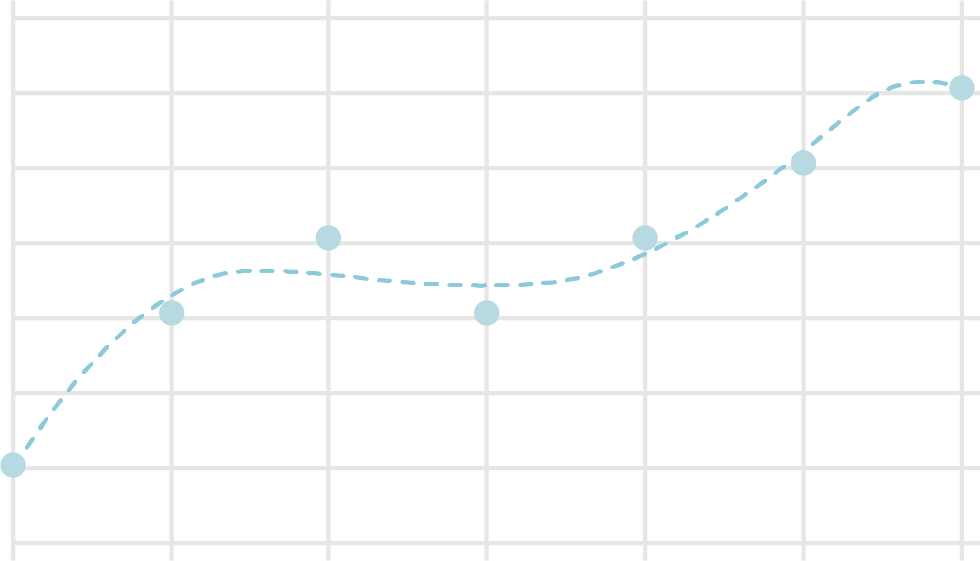
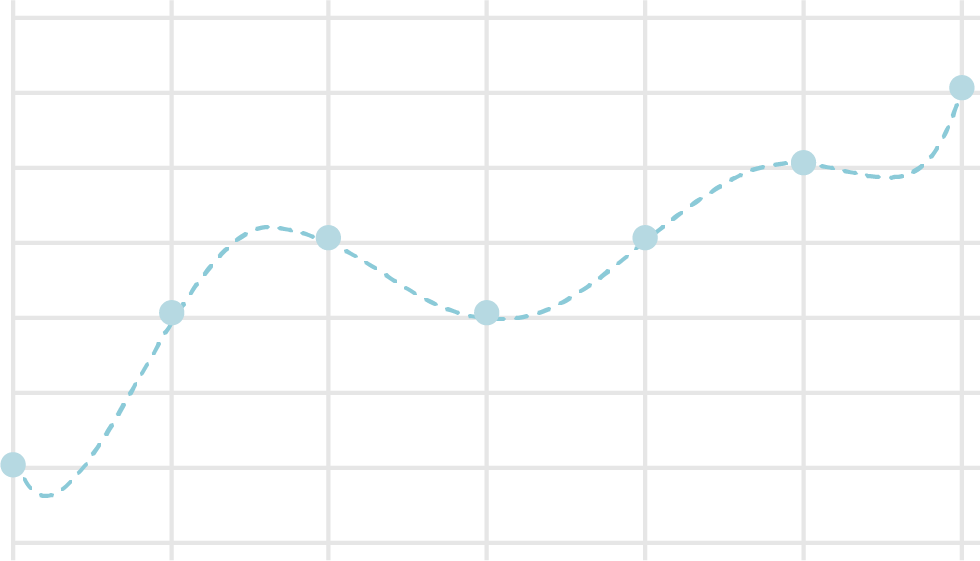
Let's see an example. The following drawings show two types of trend lines from plots on a graph. The dimension of the first graph is 3, and of the second one is 6. This example indicates 3 dimension is enough for the plots, and some values between two plots are not natural with 6.

A variety of methods to avoid overfitting are proposed. Now, we are starting from Regularization.

As you see in the following formula, we add a regularization item to loss function $E$ .

$p=1,2$ are called as L1, L2 regularization respectively. Refer to related books for the detailed explanations on why regularization is effective to avoid overfitting. An intuitive explanation is, the norm of the parameter, which results in the small range of parameter modification, is included in the loss function, and therefore the model is adjusted to the input values properly.

We often use L2 regularization for neural networks. The following is the formula.

Considering the differential result of this formula, the update formula on mini batch is as follows.

$\lambda$ is a ratio of regularization. We select a small value such as 0.01.

Now, we are going to see Dropout as another countermeasure for overfitting.

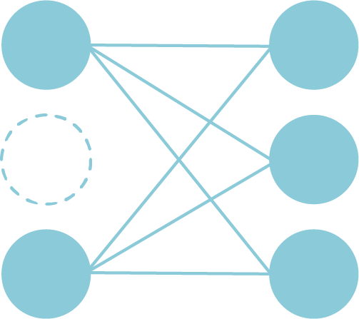
In a learning process, the system deactivates some of artificial neurons in a network randomly. Once a parameter modification is done, select deactivated items again and starts learning.

You will specify a ratio of deactivated items, which is from 0 to 1. 0.3 means 30% of the neurons are deactivated, and 70% of the items are utilized for the calculation.

Total output should reduce at $1-p$ , where the ratio is p. So, multiply $\frac{1}{1-p}$ with output values.

Keep in mind the total time for learning should be longer with dropout. You need to increase the number of learning cycles.